
Introduction
The motion energy model proposed by Adelson and Bergen (1985) has become the standard reference model for low-level, Fourier-based motion sensing in the human visual system. Its performance is consistent with a large body of published psychophysical data. The model is also elegant in its simplicity, and straightforward to implement in about 60 lines of Matlab code. The model is so easy to apply to any 1-D motion stimulus that I believe the first step in seeking to explain any low-level motion phenomenon should be to apply the model.
This web page describes the basic features of the model, and gives example Matlab code and output for the version implemented in my lab and tested against a number of psychophysical experiments (Mather & Challinor, 2009; Challinor & Mather, 2010). Initial code development was partially based on a tutorial created for a short course at Cold Spring Harbor Laboratories. All the work was supported by a research grant from the Wellcome Trust.
Model stimuli and output are represented in x-t space, illustrated in the Figure. The image of a moving car can be plotted in a three-dimensional volume which has two spatial dimensions (x and y) and a temporal dimension (t). A two-dimensional cross-section through this volume along a fixed y-position produces an x-t plot; x-position as a function of time. Movement creates oriented structure in x-t space, known as spatiotemporal orientation. The angle of tilt corresponds to the velocity of motion.
The motion energy model detects motion by detecting spatiotemporal orientation. It uses receptive fields that are oriented in x-t space. The model has an elegant way of constructing these oriented receptive fields.
The model
Here is a functional flow diagram showing the sequence of operations in the model. It can be divided into seven steps. Each step will be described in turn, listing the Matlab code for that step. For convenience, a complete script is also available, ready to run.
Step 1: Non-oriented filters
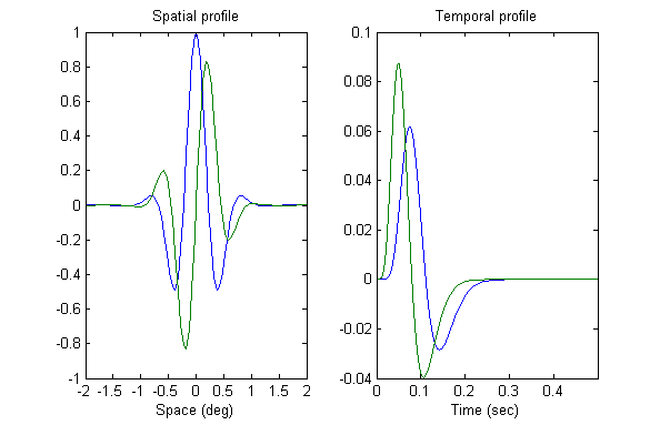
The spatiotemporally oriented receptive fields, or filters, are created from four component filters that do not themselves possess spatiotemporal orientation. Two of the spatial filters are ‘even’ functions (SE). In other words they are mirror-symmetrical about their centre. The other two spatial filters are ‘odd’ functions that do not show mirror symmetry (SO). Adelson & Bergen (1985) actually used spatial functions that were second and third derivatives of Gaussians (offering no information on the space constant of the Gaussian). Our implementation of the model uses Gabor functions – a sine wave function windowed by a Gaussian. Gabor functions offer an accurate description of cortical cell receptive fields (see Ringach, 2002). Even and odd variants are created using sine and cosine functions. Gabors have been used in other published implementations of the model (though parameter values are mostly not specified). In this implementation we use a space constant of 0.5 deg and spatial frequency of 1.1cpd, which gives a reasonable approximation to the sensitivity of the magno system (Derrington & Lennie, 1984). The Figure below shows the spatial filter profiles used in the model.
 The Matlab code to create these profiles as row vectors is listed below.
% Step 1a ---------------------------------------------------------------
%Define the space axis of the filters
nx=80; %Number of spatial samples in the filter
max_x =2.0; %Half-width of filter (deg)
dx = (max_x*2)/nx; %Spatial sampling interval of filter (deg)
% A row vector holding spatial sampling intervals
x_filt=linspace(-max_x,max_x,nx);
% Spatial filter parameters
sx=0.5; %standard deviation of Gaussian, in deg.
sf=1.1; %spatial frequency of carrier, in cpd
% Spatial filter response
gauss=exp(-x_filt.^2/sx.^2); %Gaussian envelope
even_x=cos(2*pi*sf*x_filt).*gauss; %Even Gabor
odd_x=sin(2*pi*sf*x_filt).*gauss; %Odd Gabor
%--------------------------------------------------------------------
The temporal filters in the model are biphasic, meaning that they have both a positive response phase and a negative response phase. Two variants of the temporal filter are used, one with a relatively fast response (TF), and the other with a relatively slow response (TS). The Figure above shows the two temporal profiles used in the model.
The Matlab code to create these profiles as column vectors is listed below.
% Step 1b ----------------------------------------------------------------
% Define the time axis of the filters
nt=100; % Number of temporal samples in the filter
max_t=0.5; % Duration of impulse response (sec)
dt = max_t/nt; % Temporal sampling interval (sec)
% A column vector holding temporal sampling intervals
t_filt=linspace(0,max_t,nt)';
% Temporal filter parameters
k = 100; % Scales the response into time units
slow_n = 9; % Width of the slow temporal filter
fast_n = 6; % Width of the fast temporal filter
beta =0.9; % Weighting of the -ve phase of the temporal resp relative to the +ve phase.
% Temporal filter response
slow_t=(k*t_filt).^slow_n .* exp(-k*t_filt).*(1/factorial(slow_n)-beta.*((k*t_filt).^2)/factorial(slow_n+2));
fast_t=(k*t_filt).^fast_n .* exp(-k*t_filt).*(1/factorial(fast_n)-beta.*((k*t_filt).^2)/factorial(fast_n+2));
%--------------------------------------------------------------------
The formula is modified from Adelson & Bergen (1985) Eq. 1, page 291. The only addition is the beta parameter to control the filter’s biphasic response (as used in other papers). The same formula was used by Bergen and Wilson (1985) in a study of flicker sensitivity, and seems to have its origins in early studies of temporal responses in photoreceptors (Fuortes & Hodgkin, 1964; Watson & Ahumada, 1985).
Table 1 compares the temporal filter parameters used in published implementations of the energy model. Adelson & Bergen did not use the beta parameter, and did not specify a value for the k parameter. This parameter controls the time constant of the filter, and varies in different implementations according to the time units used in the model. The current model uses units of 1 millisecond and a default value of 100 for k, with n values of 6 and 9. We have found that these values produce a good fit with the temporal properties of apparent motion.
Table 1. Temporal filter parameters |
||||
Paper |
n slow |
n fast |
k |
Beta |
Adelson & Bergen (1985) |
5 |
3 |
- |
- |
Emerson et al., (1992) |
9 |
6 |
1.5 |
0.4 |
Strout et al., (1994) |
9 |
6 |
1.5 |
0.10 & 0.72 |
Takeuchi & DeValois (1997) |
9 |
6 |
1.5 |
Vary 0-1 |
Current model |
9 |
6 |
100 |
0.9 |
Having defined the 1-D spatial and temporal profiles of the filters, we can now construct the filters as 2-D matrices. In Matlab:
% Step 1c --------------------------------------------------------
e_slow= slow_t * even_x; %SE/TS
e_fast= fast_t * even_x ; %SE/TF
o_slow = slow_t * odd_x ; %SO/TS
o_fast = fast_t * odd_x ; % SO/TF
%-----------------------------------------------------------------
The top row in this Figure shows how these filters were depicted in Adelson & Bergen’s Fig. 10. The two odd spatial filters are shown on the left (one fast and one slow), and the two even spatial filters are shown on the right (again, one fast and one slow).
Step 2: Spatiotemporally oriented filters
We now have a set of non-oriented spatiotemporal filters. They can be added or subtracted in pairs to produce a new set of linear filters that are space-time oriented, as shown in the bottom row of Adelson & Bergen’s Figure above. For example, adding the ‘odd_fast’ filter to the ‘even_slow’ filter results in a leftward-selective linear filter. In Matlab:
% Step 2 ---------------------------------------------------------
left_1=o_fast+e_slow; % L1
left_2=-o_slow+e_fast; % L2
right_1=-o_fast+e_slow; % R1
right_2=o_slow+e_fast; % R2
%-----------------------------------------------------------------
There are two leftward-tuned filters, and two rightward-tuned filters. The filters in each pair are in spatial quadrature (one is shifted by one quarter-cycle relative to the other, due to the odd/even shift).
Step 3: Convolution
Next the four filters are convolved with an x-t stimulus. First we need to define some basic parameters of the x-t space in which the stimulus resides.
% Step 3a ---------------------------------------------------------
% SPACE: x_stim is a row vector to hold sampled x-positions of the space.
stim_width=4; %half width in degrees, gives 8 degrees total
x_stim=-stim_width:dx:round(stim_width-dx);
% TIME: t_stim is a col vector to hold sampled time intervals of the space
stim_dur=1.5; %total duration of the stimulus in seconds
t_stim=(0:dt:round(stim_dur-dt))';
%--------------------------------------------------------------------
Note that the spatial and temporal sampling intervals of the stimulus (dx and dt) are inherited from the values defined in the filter code.
Next, we need a stimulus matrix. File ‘AB15.mat’ contains a matrix describing an oscillating edge image similar to that depicted in Adelson & Bergen’s Figure 15. File ‘AB16.mat’ contains a matrix describing a random dot kinematogram similar to that depicted in Adelson & Bergen’s Figure 16. To load one or the other into Matlab, use one of the following lines of code:
% Step 3b -----------------------------------------------------------
load 'AB15.mat';% Oscillating edge stimulus. Loaded as variable ‘stim’
% OR
load 'AB16.mat';% RDK stimulus. Loaded as variable ‘stim’
%--------------------------------------------------------------------
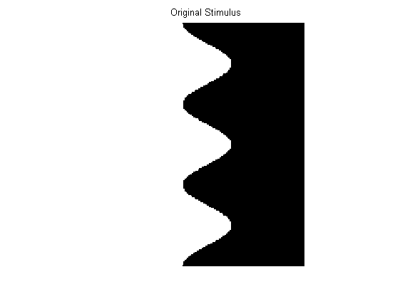
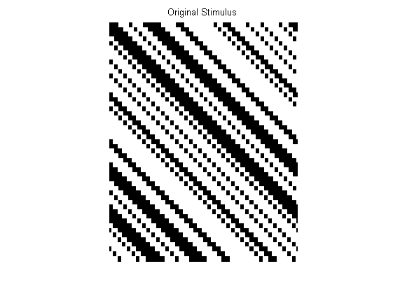
Here are these arrays as plotted as grey-level images. Alternatively you could create your own x-t stimulus matrix.
Finally, we convolve each of the four oriented filters with the stimulus array:
% Step 3c -----------------------------------------------------------
% Rightward responses
resp_right_1=conv2(stim,right_1,'valid');
resp_right_2=conv2(stim,right_2,'valid');
% Leftward responses
resp_left_1=conv2(stim,left_1,'valid');
resp_left_2=conv2(stim,left_2,'valid');
%--------------------------------------------------------------------
Note that the convolution output is a matrix that is smaller than the stimulus matrix, because it only includes ‘valid’ outputs. Each filter cannot be applied to stimulus values right near the edge of the stimulus matrix, because the filter would fall off the edge of the stimulus. (for a description of convolution, see Mather, 2009, pages 230-235, or Frisby & Stone, 2010).
Step 4: Squaring
Here we square the output of each filter:
% Step 4 -------------------------------------------------------------
resp_left_1 = resp_left_1.^2;
resp_left_2 = resp_left_2.^2;
resp_right_1 = resp_right_1.^2;
resp_right_2 = resp_right_2.^2;
%--------------------------------------------------------------------
Step 5: Normalisation
In step 5 the output of the filters is re-scaled or ‘normalised’ so that it is expressed relative to the overall level of response across all the filters. First, we calculate a single figure for total energy across the whole response array. Then the overall response in each filter is normalised by dividing it by this total.
% Step 5 ------------------------------------------------------------
% Calc left and right energy
energy_right= resp_right_1 + resp_right_2;
energy_left= resp_left_1 + resp_left_2;
% Calc total energy
total_energy = sum(sum(energy_right))+sum(sum(energy_left));
% Normalise
RR1 = sum(sum(resp_right_1))/total_energy;
RR2 = sum(sum(resp_right_2))/total_energy;
LR1 = sum(sum(resp_left_1))/total_energy;
LR2 = sum(sum(resp_left_2))/total_energy;
%--------------------------------------------------------------------
Strictly speaking, this normalisation step is not part of the original model. But evidence from cortical physiology (Heeger, 1993) and from human psychophysics (Georgeson & Scott-Samuel, 1999) indicates that normalisation does take place. Furthermore, in order to interpret the numbers produced by the model (eg. To compare directional output in different conditions) they inevitably need to be re-scaled as proportions. The normalisation computation does exactly this.
Step 6: Directional energy
Total leftward and rightward energy is calculated by summing the two filter values in each direction:
% Step 6 -------------------------------------------------------------
right_Total = RR1+RR2;
left_Total = LR1+LR2;
%---------------------------------------------------------------------
Step 7: Net motion energy
Finally, a single score for net motion energy across the whole x-t image is produced by taking the difference between the two directional scores:
% Step 7 -------------------------------------------------------------
motion_energy = right_Total - left_Total;
fprintf('\n\nNet motion energy = %g\n\n',motion_energy);
%---------------------------------------------------------------------
‘Motion_energy’ varies between -1 for pure leftwards motion, and +1 for pure rightwards motion. Zero indicates no net directional energy.
Graphical output of motion energy
Adelson & Bergen presented images of the pattern of motion energy produced by their stimuli. The following code produces an output matrix for motion energy, rather than a single global score:
% Plot model output ---------------------------------------------------
% Generate motion contrast matrix
energy_opponent = energy_right - energy_left; % L-R difference matrix
[xv yv] = size(energy_left); % Get the size of the response matrix
energy_flicker = total_energy/(xv * yv); % A value for average total energy
% Re-scale (normalize) each pixel in the L-R matrix using average energy.
motion_contrast = energy_opponent/energy_flicker;
% Plot, scaling by max L or R value
mc_max = max(max(motion_contrast));
mc_min = min(min(motion_contrast));
if (abs(mc_max) > abs(mc_min))
peak = abs(mc_max);
else
peak = abs(mc_min);
end
figure
imagesc(motion_contrast);
colormap(gray);
axis off
caxis([-peak peak]);
axis equal
title('Normalised Motion Energy');
%--------------------------------------------------------------------
Note that normalisation in this graphical code is done after taking the L-R difference, while normalisation in the earlier non-graphical code (Step 5) was done before taking the L-R difference.
Normalising before calculating net energy is mathematically equivalent to normalising after calculating net energy (as in Georgeson & Scott-Samuel, 1999) because:(L/(L+R))-(R/(L+R)) = (L-R)/(L+R). In our model depiction (Figure 2) and Step 5 we represent normalisation as being calculated first as this best reflects cortical physiology (Schwartz & Simoncelli, 2001). However, when plotting the model output we normalise after taking the L-R difference simply for convenience.
The output figure shows the distribution of motion energy. Mid-grey corresponds to zero energy, light areas contain rightwards signals and dark areas contain leftwards signals.
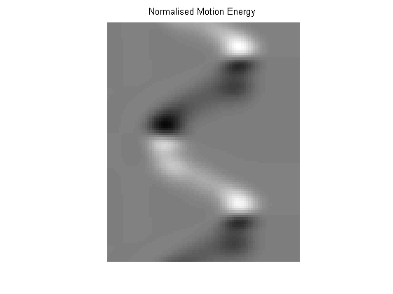
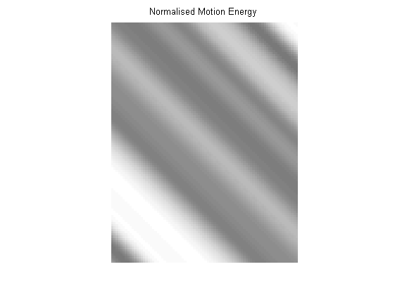
This Figure shows the response images for the two stimuli shown earlier. Compare them against the outputs shown in Adelson & Bergen’s original Figures.
References
Adelson, E. H., & Bergen, J. R. (1985). Spatiotemporal energy models for the perception of motion. Journal of the Optical Society of America, A2, 284-299.
Bergen, J. R., & Wilson, H. R. (1985). Prediction of flicker sensitivities from temporal three pulse data. Vision Research, 25(4), 577-582.
Challinor, K. L., & Mather, G. (2010). A motion-energy model predicts the direction discrimination and MAE duration of two-stroke apparent motion at high and low retinal illuminance. Vision Research, 50(12), 1109-1116. PDF
Derrington, A.M., Lennie, P. (1984) Spatial and temporal contrast sensitivities of neurones in lateral geniculate nucleus of macaque. Journal of Physiology, 357,219-240.
Emerson, R. C., Bergen, J. R., & Adelson, E. H. (1992). Directionally selective complex cells and the computation of motion energy in cat visual cortex. Vision Research, 32(2), 203-218.
Frisby, J.P., Stone, J.V. (2010) Seeing: The computational Approach to Biological Vision. Second Edition. MIT Press.
Fuortes, M.G.F., Hodgkin, A.L. (1964) Changes in time scale and sensitivity in the ommatidia of LIMULUS. Journal of Physiology, 172, 239-263.
Georgeson, M. A., & Scott-Samuel, N. E. (1999). Motion Contrast: a new metric for direction discrimination. Vision Research, 39, 4393-4402.
Heeger, D. J. (1993). Modeling simple-cell direction selectivity with normalized, half-squared, linear operators. Journal of Neurophysiology, 70(5), 1885-1898.
Mather, G. (2009) Foundations of Sensation and Perception. Second Edition. Psychology Press.
Mather, G., & Challinor, K. L. (2009). Psychophysical properties of two-stroke apparent motion. Journal of Vision, 9(1:28), 1-6. PDF
Ringach, D. L. (2002). Spatial structure and symmetry of simple-cell receptive fields in macaque primary visual cortex. J. Neurophysiol, 88, 455-463.
Schwartz, O., & Simoncelli, E. P. (2001). Natural signal statistics and sensory gain control. Nature Neuroscience, 4(8), 819-825.
Strout, J. J., Pantle, A., & Mills, S. L. (1994). An energy model of interframe interval effects in single-step apparent motion. Vision Research, 34, 3223-3240.
Takeuchi, T., & De Valois, K. K. (1997). Motion-reversal reveals two motion mechanisms functioning in scotopic vision. Vision Research, 37, 745-755.
Watson, A.B., Ahumada, A.J. (1985) Model of human motion sensing. Journal of the Optical Society of America, A2, 322-342.